You will find an Excel template for shift and work schedules.
If you manage your shift schedule in Excel, it's convenient because it allows you to calculate the working hours automatically.
If you are managing a large number of staff members in a handwritten shift schedule, it would be a hassle to edit it every time there is a correction, so take this opportunity to use an Excel template.
You can download monthly, weekly or daily shift schedule templates.
Shift schedule excel template
There are excel templates for a month, a week, and a day. You can use these templates as a base and modify them to make them easier to use.
Click to view a larger image.
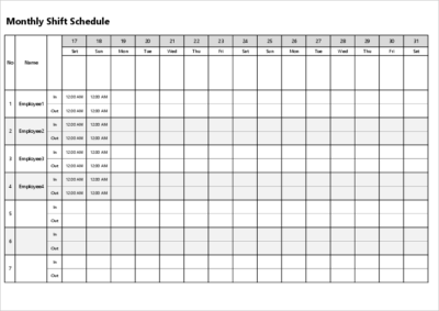
Monthly shift schedule
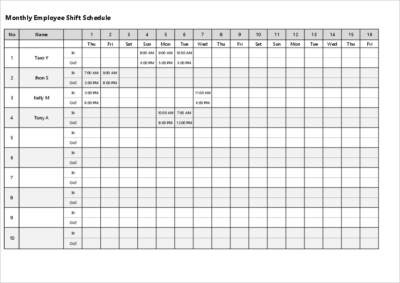
Enter a date in the "Period Start Date" field and the date and day of the week for the month will be automatically set.
To use the system, enter the start time in the "In" column and the end time in the "Out" column. There is no automatic calculation of working hours.
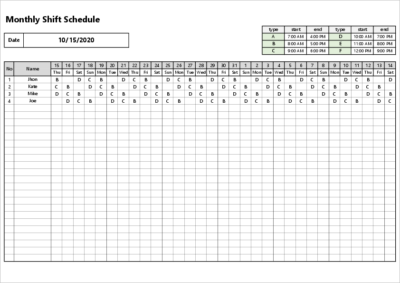
If you feel the table is too small, change the height of the rows to reduce the number of staff members.
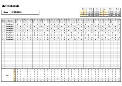
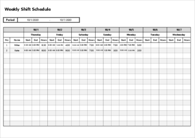
The difference is that it has a total column at the bottom, and it calculates the working hours automatically. You can see the number of people from A to F per day.
Weekly shift schedule
Daily shift schedule
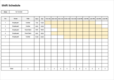
The color of the chart is set in conditional format, so if you want to change the color of the chart, select each employee's cell at 7 o'clock and change it from "Conditional Format".
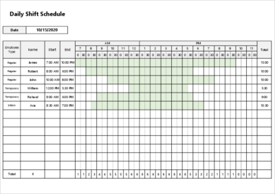
This template is almost the same format as Template "Shift02", but "Shift02" can be created by hourly increments, while "Shift06" can be created by 30-minute increments. When you enter the start and end time, the system will automatically calculate the number of people per hour and work hours. The chart is not created automatically, so you have to fill in the shift hours yourself.
How to make a shift schedule in Excel
If you want to make your own Excel shift chart instead of a template, here's how to make a shift chart.
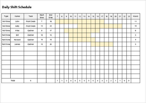
There are various ways to make a shift chart, but in this article, I will try to create a shift chart like the one below, which automatically calculates the number of people in a shift for a day.
The automatic calculation is based on the number of people in the shift and the number of hours worked that day.
1. Adjust the size of the cell
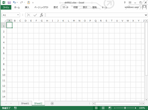
The first thing to do is to adjust the size of the vertical and horizontal cells in Excel.
By default, the width is too long, so when you create a calendar for the front part of the shift table, you can't get enough dates.
Let's create a 30 pixels wide by 30 pixels high.
2. Create a table of names and calendars
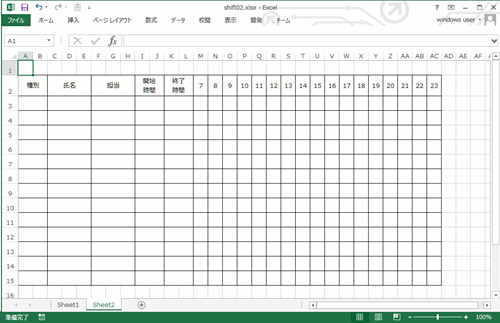
We'll design the whole thing later, and create a table of people and hours for the shift.
In the sample, I made a table with the "type", "name", "task", "start time", "end time", and 7:00-11:00 pm to distinguish between full-time and part-time employees.
3. Create a column for the total number of people
In this case, we're going to calculate the number of hours each person works and how many people come to work during those hours, so we're going to create a column to display the calculation results in the right-hand side and bottom of the Excel table we just created.
4. Automatic calculation of work hours
Let's start by calculating the work hours on the far right. Working hours are calculated from the start and end time of the job.
End time - Start time gives you the work hours, so enter =K3-I3 in the first work hours cell.If you don't do this, you will also get a "0" in the column where there is no person in charge, so don't display it.
=IF(K3="","",K3-I3)
I used the IF function in Excel to create a formula that says that if K3 doesn't have any data in it, it won't show anything in the cells.
If you copy the formula cell you created at the top to the bottom, the formula will be in all the cells of the working hours.
5. Automatic calculation of the number of people per hour
Next, we calculate how many people are shifted at a particular time.The Excel function we will use is COUNTIFS.
The COUNTIFS function calculates the number of people who match multiple search criteria within a specified range.In this case, we count whether the start and end times for each rep are within the relevant time.
=COUNTIFS(First person's start time: last person's start time, "<= the relevant time",First person's end time: last person's end time, "> the relevant time")
Calculate in
For example, if it's 7 o'clock
=COUNTIFS(I4:I16,"<=7",K4:K16,">7")
will calculate the number of people who are in at 7:00.
If you copy this cell to the right, you can get the number of people at each hour.
6. Align the design
Finally, align the design so that it is easy to see. Add a title, date and time field and color to the Excel and you're done. Inserting or deleting cells will not break the function you just created, so it's okay.
Summary
We've introduced you to how to make a shift chart and attendance chart, as well as an excel template.
I'm sure there are a lot of stores that create shift charts by hand, but once you create a template in Excel, you can automatically create dates and days of the week, making it easier to print out the shift chart every month.
If you want to revise or make a more user-friendly shift chart, you can easily do so once you learn some Excel, so try using the template to create your own shift chart.


